当前位置: 网站首页 >> 智库成果 >> SG论文 >> 正文

李强：CORRUPTION TAKES AWAY HAPPINESS

发布者： [发表时间]：2019-03-08 [来源]： [浏览次数]：

Running head: CORRUPTION TAKES AWAY HAPPINESS

Corruption Takes Away Happiness:

Evidence from a Cross-National Study

Qiang Li, Ph.D., corresponding author

Associate professor in Economics

Public Administration School, Guangzhou University, China

qiangliriem@gmail.com

Lian An, Ph.D.

Professor in Economics

School of Business, Hubei University, China

and

Coggin College of Business, University of North Florida, USA.

lian.an@unf.edu

Corruption Takes Away Happiness:

Evidence from a Cross-National Study

1. Introduction

The world has witnessed a remarkable decline in average subjective well-being since 2005 (Figure 1). Identifying the sources of people’s well-being is important (Frey and Stutzer, 2000)because a primary human objective is to achieve greater happiness for a greater number of people (Brülde, 2010; Veenhoven, 2010). Researchers have long been trying to explain the determinants of happiness.[1]Multiple studies have shown many economic factors affect happiness, including gross domestic product (GDP) per capita, unemployment, and lack of inflation (Altindag and Xu, 2017; Oswald, 1997;Tavits, 2008). Frey and Stutzer (2002)recently proposed that the kind of political system people live in influences their happiness. A particularly important factor in the political system that affects happiness is corruption.

Corruptionis defined as misuse of public power for private gains (Lambsdorff, 2007). Corruption affects happiness for at least the following four reasons. First, corrupt institutions produce mistrust among citizens (Rothstein, 2010; Tay, Herian, and Diener, 2014), and there is evidence that interpersonal trust increases happiness (Graafland and Compen, 2015; Growiec and Growiec, 2014; Hommerich and Tiefenbach, 2018; Puntscher et al. 2015;Ram, 2010). Second, corruption curbs investment and thereby lowers economic growth (Coggburn and Schneider, 2003; Mauro, 1995; Mo, 2001), which may further affect subjective well-being (Sacks et al. 2010). Third, corruption aggravates income inequality (Glaeser and Saks 2006), which influences well-being (Alesina et al. 2004;Brockmann et al. 2009;Graafland and Lous 2017; Oishi et al. 2011;Schröder 2018;Tavor et al. 2017). Fourth, corruption distorts the composition of government expenditure by devoting less to the education sector (Mauro, 1998),which would enhance happiness, while devoting more to the military sector (Gupta et al. 2001),which does not enhance happiness.

For a direct visual inspection of the link between corruption and happiness, we constructed a scatter plot of happiness (2014) versus corruption (2014) in Figure 2. The happiness index is from the World Happiness Report, by the United Nations Sustainable Development Solutions Network. We used the corruption perception index (CPI) from Transparency International (TI) to measure corruption. It clearly shows a negative relationship between corruption and happiness: the higher the corruption, the less the happiness.

While the scatter plot reveals the correlation between corruption and happiness, it cannot answer the causal relationship between the two variables: does corruption lead to lower subjective well-being? Furthermore, the causal effect of corruption on subjective well-being is not as clear-cut as it first appears. There are two concerns. First, the endogeneity issue has not been well addressed (Frey and Stutzer, 2002). Inglehart(1999)noted that it remains open whether democracy fosters life satisfaction or whether high satisfaction with life in a population increases the legitimacy of the political regime in power, thus fostering democracy. Frey and Stutzer further stated that attitudes favoring democracy and life satisfaction reinforced each other. One may infer a reverse causality between corruption and happiness from their observation. However, reverse causality has not been well addressed in the literature. For example, while Welsch (2008),Tavits (2008), and Ott(2010a)all found corruption to be negatively correlated with happiness and admitted that higher happiness was more likely to lead to lower corruption, they all left reverse causality unaddressed. Coincidentally, by using individual-level datasets in China and Africa,Graham (2011), Wu and Zhu (2015), and Sulemana et al. (2017)found that being a victim of corruption was correlated with lower happiness.[2]They did not solve the endogeneity issue, either. Ott (2010b)queried whether the corruption and happiness correlation was a consequence of causality. It is only recently, with Arvin and Lew (2014) and Sulemana (2015),that researchers have begun to specifically address reverse causality in estimating the effect of corruption on happiness. However, the validity of their instrument variables (IV) is open to question.[3]

Second, corruption is quite hard to measure because the definitions of corruption vary across countries and over time. Therefore, the measurements of corruption might not be free from error, and only a few studies have taken measurement error into consideration. For example, León et al. (2013)tried to address the measurement error in corruption and happiness using individual data in Spain and found them to be negatively correlated. However, the authors did not address the reverse causality issue.In sum, the causal relationship between corruption and happiness is far from well established, and this paper intends to explore this causal relationship.

This paper addresses the endogeneity issue by adopting a novel IV. In our research, we employed the local traditional democracy of around 500 years ago as an IV for corruption in the 21st century. Contemporary economic and political development have deep roots in history. For example, Acemoglu et al. (2001)found that colonial origin influenced comparative economic development. Nunn and Wantchekon (2011)found that the slave trade of more than 400 years ago led to the interpersonal mistrust in Africa. Recent research by Giuliano and Nunn (2013)showed that local traditional democracy in the preindustrial period was correlated with current corruption, using preindustrial ethnographic data of over 100 ancestral characteristics for 1,265 ethnic groups in Murdock’s(1967)Ethnographic Atlas. Because preindustrial local traditional democracy is correlated with current corruption and uncorrelated with unobservable omitted variables, and it should not affect contemporary subjective well-being other than through its effect on current corruption, it serves as a valid IV for current corruption. We thus used the local traditional democracy level from around 500 years ago as an IV for current corruption.

In addressing the difficulty in measuring corruption, we followed Li et al. (2018)in using different sources of corruption to cross-check the robustness of the results. Specifically, in addition to the commonly used CPI from TI, we adopted Freedom from Corruption from the Heritage Foundation, Control of Corruption from the World Bank’s Worldwide Governance Indicators (WGIs), and the Bayesian Corruption Index (BCI) from Sherppa Ghent University to cross-check the validity of our corruption measurement.

To preview the results, we noted that societal perceptions of corruption have a significant adverse influence on general well-being. Specifically, a 10-point increase in corruption on the perception index on a 0–100-point scale (i.e., a government becomes more corrupt) would cause a 0.23-point decrease in national average scores for subjective well-being on a 0–10-point scale. This finding is both statistically significant and sizeable in economic meaning. A simple calculation indicated that the unemployment rate had to decrease by 9.2% to keep the national average subjective well-being unchanged if the CPI decreased by 10 points. Further investigation showed that corruption had a significant effect in democratic or high-income countries only. The results were robust for alternative measures of corruption and happiness, estimation methodologies, and excluded influential outliers.

This paper contributes to the literature on this topic in the following ways: 1) it provides a more consistent estimator of a corruption–happiness relationship to the literature by using a novel IV; 2) the IV used in this paper can also be generalized to the relevant literature; 3) the paper further explores the potential channels through which corruption affects subjective well-being.

This paper is structured as follows. Section 2 presents the methodological framework, including the description of the data and the model. This section also addresses the endogeneity issue by using instruments. Section 3 presents the results. Section 4 extends the analysis by testing the robustness of the results, particularly by making use of alternative indices of corruption and subjective well-being. Section 5 concludes and suggests avenues for future research.

2. Methodological Framework and Data

To estimate the effect of corruption on happiness, we specified the following model:

Y_i=α+β*CPI_i+X_i’γ+ε_i, (1)

where dependent variable Y is the national-level average scores in country ifor subjective well-being taken from the World Happiness Report, which ranks 155 countries by their happiness level. The World Happiness Report is a landmark survey of the state of global happiness. The first report was published in 2012, the second in 2013, and the third in 2015.The survey asked roughly 3,000 respondents in each country to evaluate their current lives on a scale where 0 represents the worst possible life and 10 the best possible. There is skepticism about interpreting happiness scores as cardinal numbers, butKahneman(1999)showed that this may be less problematic at a practical level than at the theoretical level (Frey and Stutzer, 2000).Di Tella et al. (2001)also indicated that assuming cordiality or cardinality of happiness scores had little impact on empirical results. In addition, the cardinal numbers we adopted can allow one to compute average happiness at the national level. This has an advantage over the micro-approach based on individual happiness levels because the unobserved heterogeneity across individuals can even out, and cross-national heterogeneity can be easily captured by controls on cultural, demographic, and institutional situations.

The CPI from country-based survey data collected by various institutions and published by TI is a composite index based on a 0–100 point scale in which a score of 100 indicates very little corruption and a score of 0 indicates very high corruption in the public sector. It is a measure based on indicators obtained from subjective data and on a “poll of polls” with a range of corruption measures from up to 15 different sources, including the opinions of experts and business executives. The measures are aggregated to reduce measurement error. Precisely measuring corruption is difficult, however, so to make our results more robust, we also used three other corruption measures: the Free from Corruption from the Heritage Foundation, Control of Corruption from the World Bank, and the BCI from Sherppa Ghent University.

X is a set of control variables, including GDP per capita growth rate, capital stock, unemployment rate, population weighted average exposure to PM2.5,[4]working age population, religious fractionalization,[5]ethnic fractionalization,[6]and language fractionalization.[7]These variables have been commonly used in the literature.

We did not include GDP and capital stock simultaneously because influences that originate from a country’s overall economic development are well captured by its capital stock (Lambsdorff, 2003). We used GDP growth instead because it is an indicator of a country’s economic potential, which is important for that country’s happiness and well-being.

There is overwhelming evidence that the unemployment rate takes a heavy toll on life satisfaction (Helliwell et al. 2017;Wang and Wong 2014). As Akerlof and Shiller (2010)put it, “I have always thought of unemployment as a terrible thing. A person without a job loses not just his income but often the sense that he is fulfilling the duties expected of him as a human being.” We thus included unemployment rate as a control variable.

The previous literature has rarely included environmental indicators in the happiness function. With the development of the world economy and a deteriorating environment, air pollution is no longer negligible for a country. The World Health Organization (WHO) has estimated that 3 million premature deaths per year can be attributed to the effects of atmospheric pollution, and the long-term exposure to PM2.5 reduces life expectancy by 8.6 months in the European Union. Zhang et al. (2017a)found that air pollution reduces hedonic happiness. Zhang et al. (2017b)also found that people on average were willing to pay $42 (or 1.8% of annual per capita income) per year per person for a 1% reduction in PM2.5. Therefore, not including air pollution would lead to an omitted variable bias. This paper controls for population weighted exposure to PM2.5 (3-year average), which originally comes from the Global Rural Urban Mapping project, v.1, at the NASA Socioeconomic Data and Applications Center, hosted by the Center for International Earth Science Information Network (CIESIN) at Columbia University. This indicator is then converted to a scale of 0–100 by simple arithmetic calculation, with 0 being the farthest from the target and 100 being closest to the target defined by established scientific consensus, as is the case with WHO’s recommended average exposure to fine particulate matter (PM2.5).

The working-age population makes up a proportion of the total population. It was included to control the age structure of a nation because the data on the average age are not available. According to Helliwell (2003), age is an important predictor of individual happiness. The arguments can be made both ways. On the one hand, stress is highest for the working-age population because they have more life chores, such as raising kids and caring for old parents. Oswald (1997)and Frey and Stutzer (2002) found that middle-aged individuals express less happiness than the very young, who face fewer financial pressures or family commitments, or older citizens who are well established. On the other hand, the working age is the strongest and most healthy stage in the life cycle. Physical and mental condition both reach their peak in one’s life then, and thus one may argue that the working age is the happiest age in life.

Three fractionalization indices are included to control the impact from cultural diversity on life satisfaction and happiness (Hinks, 2012). According to Shleifer and Vishny (1993), many ethnolinguistic fractionalized countries tend to have more dishonest bureaucracies. Also, cross-country research by Mauro (1995), Montalvo and Reynal-Querol (2005), and Li et al. (2018)indicated that ethnolinguistic diversity, captured by ethnolinguistic fractionalization, can have connotations for quality of governance, economic growth, and health status, which have a far-reaching impact on subjective well-being and happiness. The same reasoning applies to other fractionalization indices. More recently, fractionalizations have been included in models of trust, health, and the like, and to a lesser extent in well-being and happiness literature.

Our data comes from the Quality of Government (QOG) dataset andGiuliano and Nunn (2018). The QOG dataset drew on and compiled a number of freely available data sources, including the World Bank, TI, and aggregated individual-level data (Teorell et al. 2017). Giuliano and Nunnconstructed an Ancestral Characteristics Databasemeasuring the cultural and environmental characteristics of the preindustrial ancestors of the world’s current population, using data originally from the Ethnographic Atlas,which provides information on the preindustrial characteristics of 1,265 ethnic groups. Since the preindustrial local traditional democracy did not change over time within the same country and there are missing values in some control variables, 126 countries in 2014 were finally used in this analysis. When doing a robustness check, we also took advantage of the panel structure of the data set in running fixed effect and random effect models.

Table 1 presents the descriptive statistics of all variables. We give the mean value of the main variables divided into several groups, represented by the 25th, 50th, 75th, and 100th percentiles of the CPI. The mean CPI was 44.64, and the average subjective well-being was 5.45. It is interesting to note that as we moved along to the higher quartile of CPI, indicating less corruption, the mean subjective well-being increased, which indicates that corruption and happiness might be negatively correlated. However, the capital stock, PM2.5, unemployment rate, and religious fractionalization did not show the same pattern. For more detail, please see Table 1.

3. Baseline Result

We first ran a regression of our model given in Equation (1) using the method of ordinary least square (OLS) with and without control variables and have reported the results in Columns 1 and 2 of Table 2. The coefficients of CPI on happiness were 0.039 and 0.026 without and with other control variables, respectively, and they were highly significant at 1%. This implies that a 10-point increase in the CPI (0–100-point scale) is associated with a 0.26-point increment of the national average of subjective well-being. This indicates that corruption is negatively correlated with the general subjective well-being of a country.

The OLS estimations are not free from bias caused by reverse causality. We employed the local traditional democracy of around 500 years ago as an IV for corruption in the 21st century to address the endogeneity issue. As discussed in the introduction, preindustrial local traditional democracy is correlated with current corruption and uncorrelated with unobservable omitted variables, and it cannot affect contemporary subjective well-being other than through its effect on current corruption. It therefore serves as a valid IV for current corruption. The first-stage regression results indicated that the preindustrial local traditional democracy was highly correlated with the current CPI. We reported the detailed results on the first-stage regression in Table A1 in the appendix A. To further test the validity of our IV, we carried out an under-identification test and a weak identification test, and the IV passed both. Specifically, we rejected the null hypothesis of under-identification, and the test indicated that the significance level was distorted from 5% to less than 10% in two-stage least square (2SLS). We have reported these tests results in Columns 3 and 4 in Table 2.

We then ran a regression of our model given in Equation (1) using the 2SLS method with and without control variables. We reported the results in Columns 3 and 4 of Table 2. The coefficients of CPI on happiness were 0.042 and 0.023 without and with other control variables, respectively, and they were highly significant at the 5% significance level. This indicates that a 10-point increase in the CPI can cause the national average of subjective well-being to increase by 0.23 points.

Our 2SLS and OLS estimators are both significant statistically and sizeable in economic meaning. Taking the unemployment rate as an example, we calculated how much the unemployment rate must decrease to keep the national average subjective well-being constant when the CPI decreases by 10 points (i.e., a government becomes more corrupt). A simple calculation showed that the unemployment rate had to decrease equivalently by 9.2% to keep the national average subjective well-being unchanged if a government became more corrupt by 10 points. Taking Greece, Italy, and Brazil as examples to illustrate what a 10-point decrease in CPI means, we can see that their CPI was 43 in 2014, which is very close to the sample average. If we move along the CPI scale to 33, we find the countries Albania, Ecuador, Ethiopia, and Malawi. Our results imply that if we could arbitrarily move people from Albania to Italy, or Ecuador to Greece, these emigrations could tolerate a 9.2% higher unemployment rate to keep their subjective well-being the same as in their native Albania or Ecuador.

One may notice that the coefficient of corruption does decrease when the IV method is adopted compared to the OLS. Basu(2015)found that the OLS would overestimate the true effect whenever there was reverse causality.The 2SLS estimator was 0.023, smaller than the OLS estimator of 0.026, which is consistent with Basu’s prediction. However, the interpretation should be approached with caution because the difference between the 2SLS and OLS estimators is not significant, due to the larger standard error of the 2SLS estimator than of the OLS estimator.[8]

In sum, our key findings were that the coefficients for corruption in different specifications were significantly positive, so reducing corruption must be helpful in increasing people’s feeling of happiness. These results are consistent with most previous literature. According to Rothstein and Stolle (2003), incorrupt and effective governmental institutions have been shown to produce trust between citizens, and there is evidence that interpersonal trust increases happiness (Helliwell and Huang 2008; Spruk and Kešeljević 2016). It is also possible that corruption causes people to feel unhappy by curbing investment, distorting government expenditure, and aggravating income inequality.

The estimates of other control variables were basically consistent with our expectations. We found that increasing the unemployment rate would reduce national-level subjective well-being, which is consistent with Gonza and Burger (2017). We also found that increasing capital stock would increase subjective well-being and that when the environment improved, as measured by less exposure to PM 2.5, the general level of subjective well-being increased, which is consistent with the prediction of Heylighen and Heylighen(2000). GDP growth does not contribute significantly to the general subjective well-being. This may sound counterintuitive at the first glance, but it is not without reason. GDP growth is typically exemplified by so-called “social regrettable” outcomes such as pollution, crime, and divorce. For example, more expenditure on jails indicates a decrease in well-being but an increase in GDP. Thus, it is not surprising if GDP growth was not shown to be significant in explaining happiness. We found that a working-age population has a significant positive impact on happiness. The higher the proportion of the working-age population in a country, the higher its subjective well-being.

In this study, religious fractionalization had a significant positive impact on subjective well-being, which differed from Hinks’s (2012)and Mookerjee and Beron’s(2005)conclusion that religious fractionalization was correlated with lower life satisfaction. Hinks explained that the bond within a religious group was outweighed by the lack of bridging between religious groups. Too much within-group bonding, he said, could result in a polarized position between groups that caused the life satisfaction of all groups to decline. However, we found that religious fractionalization could significantly increase subjective well-being. We deemed that the index also captured the freedom to follow a religion of their choice. While the polarized position between groups might decrease life satisfaction, the freedom to follow religion would make people feel happy. In Table 7 below, we identify freedom of religion as one of the valid potential channels through which corruption affects subjective well-being.

Ethnic fractionalization significantly decreases well-being. Our results were consistent with Putnam (2007)and Alesina and La Ferrara (2002), who found that ethnic diversity was negatively correlated with social capital or cohesion measured by trust, altruism, reciprocity, cooperation, and civic engagement, and thus overall well-being. However, some literature has found ethnic diversity to have a positive effect on the well-being of a country, such as Akayet al. (2017). Language fractionalization does not have a significant impact on life satisfaction. Hinks (2012)concluded similarly that ethnolinguistic fractionalization does not correlate with life satisfaction.

4. Robustness Check

The index on corruption and happiness relates to subjective perceptions of people and country analysts, which are usually difficult to measure. Still, the concern that personal perceptions may overshadow responses and introduce measurement error is hard to discount. In addition, the results may be influenced by some extreme observations and different model specifications. For these reasons, we performed several robustness checks regarding: (a) alternative measures of corruption; (b) alternative measures of subjective well-being; (c) excluding influential outliers; (d) alternative models; and (e) heterogeneity of the corruption effect.

Our baseline analysis adopted the commonly used measure from TI. There are several other agencies compiling the corruption index, thus providing us with the opportunity to use different measurements of corruption to cross-check the robustness of our primary results. Of these, we adopted three: Freedom from Corruption, Control of Corruption, and the BCI.

The Freedom from Corruption measure relies on TI’s CPI. It measures the level of corruption in 152 countries to determine the freedom from corruption scores of countries that are also listed in the Index of Economic Freedom. In scoring freedom from corruption, the index converts the raw CPI data to a scale of 0–100 by multiplying the CPI score by 10.[9]For countries not covered in the CPI, the freedom from corruption score is determined by using the qualitative information from internationally recognized and reliable sources. This procedure considers the extent to which corruption prevails in a country. The higher the level of corruption, the lower a country’s score.

The Control of Corruption measurement comes from the World Bank’s WGIs. It conventionally defines corruption as the exercise of public power for private gain, which includes various formats of corruption ranging from the frequency of additional payments needed to get things done, to the effects of corruption on the business environment, measuring grand corruption in the political arena, and the tendency of elite forms to engage in “state capture.” It ranges from approximately -2.5 (weak) to 2.5 (strong) governance performance.

The BCI lies between 0–100 with an increase in the index corresponding to a rise in the level of corruption. This is a difference between CPI and BCI, where an increase in the index means that the level of corruption has decreased. More specifically, 0 corresponds to a situation in which all surveys indicate that there is absolutely no corruption, and 100 represents the worst possible level of corruption. Methodologically, it is closely related to Control of Corruption because the procedure to construct the BCI is an augmented version of the procedure to construct WGIs (Standaert, 2015).

Table 3 displays the results using alternative measures of corruption as a robustness check. To save space, we reported the estimates on corruption for OLS and IV specifications with and without other control variables. The results are robust across the different measures of corruption.

Our second robustness check addressed the concern with respect to measures of happiness, for which we used the “inequality of happiness” of the nations proposed by Kalmijn and Veenhoven (2005)and Lin et al. (2017), and the “happy life-expectancy” proposed by Veenhoven (1996)as alternative measures. “Inequality of happiness” measures the degree to which citizens in a country differ in their enjoyment of life.[10]“Happy life-expectancy” indicates the length of a happy life a typical person leads in a country.[11]Our results are in Table 4. The results regarding these alternative measures of happiness were clearly robust.

The third robustness check addressed the concern that our results might be driven by outliers, as Figure 2 shows that some countries clearly appear as outliers. For example, Afghanistan, Burundi, and Togo have the lowest CPI and lowest average happiness scores of the countries we have researched, raising the question as to whether such outliers may influence our baseline results. Next, we checked to see if our results were robust to influential outliers. The first sensitivity test estimated our baseline specification with the standard full set of control variables but excluded the 10 least corrupt and 10 most corrupt countries. We report the results in Columns 1 and 2 of Table 5, respectively. The results were robust to excluding such outliers. We also adopted a more systematic approach to deal with influential observations and remove them using each observation’s difference of the estimated coefficient (DFBETA) for the CPI when the observation was included and when it was excluded from the sample. Following Belsleyet al.(1980), observations with |DFBETA|>2/ are omitted, where N is the number of observations, which is 126 in our case. Results are presented in Column 3 of Table 5. Figure 2 also indicates that only a small fraction of observations were particularly influential because the CPI is skewed to the left. We addressed this by performing a zero-skewness Box-Cox power transformation on the CPI to obtain a measure with zero-skewness of corruption that did not feature influential and outlying observations. Regression results are reported in Column 4 of Table 5. Clearly, in all four tests in Table 5, the coefficients on the CPI remained positive and statistically significant, confirming that outliers would not influence our results, and the conclusion that corruption takes away happiness stands on its own.

The fourth robustness check considered alternative estimation strategies. We carried out a robustness check with respect to different estimation methodologies by taking advantage of our panel data. Specifically, instead of employing an instrumental variable, we used fixed effect and random effect models to difference out unobservable country fixed effect. We used data from 2004–2014, during which time CPI and happiness information was available. Results are presented in Table 6. The results were robust to a different specification with and without control variables. Overall, the results provide robust evidence that societal perceptions of corruption are detrimental to subjective well-being.

The baseline regressions assume that corruption has the same impact on different countries. It would be more realistic if we allowed that corruption has a different impact on happiness for different countries. We therefore followedOtt(2010b)to divide countries into low- and high- income countries and Boix et al. (2013)to divide countries into nondemocratic and democratic countries. Table 7 reports results from this experiment. The first two columns show that the corruption coefficient is significant in high-income countries while insignificant in low-income countries, which indicates that corruption has a significant impact on high-income countries only. This finding is consistent with Arvin and Lew (2014). As shown in the last two columns in Table 7, the coefficient is significant in democratic countries while insignificant in nondemocratic countries, which indicates that corruption has significant influence only in democratic countries. This finding is consistent with Ott (2010b)and similar to Rode (2013). From the results, we infer that corruption in low-income or nondemocratic countries may be deep-rooted in society and indiscernible among the multitude of depravities; therefore, corruption in these countries has no effect on happiness, and vice versa.

After establishing the link between corruption and happiness, we next moved to investigate through what channels corruption affects happiness. Because corruption includes many different types of behavior, the channels for its adverse effect on happiness can be manifold. We could not exhaust all the channels, but we did investigate several key channels that had data availability for the year 2011: freedom of religion, freedom of expression, equal opportunity, and freedom of assembly and association. We first regressed each of the variables on corruption; our results are shown in Table 8, Columns 1–4. All the coefficients of CPI are highly significant, indicating that corruption is correlated with all four of these channels. We then regress subjective well-being on CPI and all four channels together, as is presented in Column 6. In comparison with Column 5, which runs subjective well-being on CPI only, the coefficient of CPI decreased substantially from 0.035 to 0.015, and the coefficients on equal opportunity and freedom of assembly and association are still highly significant. Combining all the results, it is clear that freedom of religion, freedom of expression, equal opportunity, and freedom of assembly and association are among the channels through which corruption affects happiness.

5. Conclusion and Discussion

Contemporary empirical investigation has found an ambiguous link between corruption and GDP or other economic variables, which are not genuine indicators of welfare per se. As such, the link between corruption and happiness is blurred. Motivated by this void in the literature, the study clarifies this link by using a newly assembled panel data set consisting of perception on corruption and subjective well-being. For the first time in corruption–happiness literature, we have addressed endogeneity by using local traditional democracy around 500 years ago as an IV. We carried out various robustness checks, and the negative associations between corruption and subjective well-being were significant in a variety of regressions. We obtained repeated support for the theory that corruption lowers the well-being of a country. In addition, we identified several key channels through which corruption influences well-being (i.e., freedom of religion, freedom of expression, equal opportunity, and freedom of assembly and association). Corruption had a significantly adverse influence on these variables, which were also important for a country’s well-being.

One practical implication of this study is that societal corruption should be a matter of concern to academics, governments, and policy makers because it lowers national well-being. In countries with a history of corruption, the necessity to mitigate the psychological effects of corruption may be especially paramount. Continued research may endeavor to refine and further validate measurement of corruption and ultimately contribute to interventions designed to combat its detrimental impacts.

This paper has several limitations. First, while our instrument is novel in that it connects historical democracy with current corruption, it is time invariant, which prohibits us from taking advantage of the available panel dataset. Second, the difference between our OLS and 2SLS estimator on the CPI is indiscernible, which questions the validity of our IV. Even if previous literature has shown that preindustrial democracy is correlated with current corruption, there are still possibilities that its evolution may directly affect subjective well-being or that it is correlated with idiosyncratic factors of specific countries that are confounded with current corruption,[12]invalidating the eligibility of this IV. Third, the national average score of subjective well-being is highly persistent, which necessitates the use of dynamic panels to capture its persistence. Therefore, future research could use the available panel dataset and use the general method of moments to further explore the relationship between corruption and happiness.

References

Acemoglu, D., Johnson, S., & Robinson, J. A. (2001). The colonial origins of comparative development: An empirical investigation. American Economic Review, 91(5), 1369–1401.

Akay, A., Constant, A., Giulietti, C., & Guzi, M. (2017). Ethnic diversity and well-being. Journal of Population Economics, 30(1), 265–306. Retrieved June 19, 2018, from http://link.springer.com/10.1007/s00148-016-0618-8

Akerlof, G., & Shiller, R. (2010). Animal Spirits: How Human Psychology Drives the Economy, and Why It Matters for Global Capitalism. Princeton University Press. Retrieved from https://econpapers.repec.org/RePEc:pup:pbooks:9163

Alesina, A., & La Ferrara, E. (2002). Who trusts others? Journal of Public Economics, 85(2), 207–234.

Alesina, A., Di Tella, R., & MacCulloch, R. (2004). Inequality and happiness: Are Europeans and Americans different? Journal of Public Economics, 88(9–10), 2009–2042.

Altindag, D. T., & Xu, J. (2017). Life Satisfaction and Preferences over Economic Growth and Institutional Quality. Journal of Labor Research, 38(1), 100–121.

Arvin, M., & Lew, B. (2014). Does income matter in the happiness-corruption relationship? Journal of Economic Studies, 41(3), 469–490. Emerald Group Publishing Limited. Retrieved September 23, 2017, from http://www.emeraldinsight.com/doi/10.1108/JES-02-2013-0024

Basu, D. (2015). Asymptotic Bias of OLS in the Presence of Reverse Causality( No. 179). Economics Department Working Paper Series. Retrieved June 13, 2018, from https://scholarworks.umass.edu/econ_workingpaper/179

Belsley, D. A., Kuh, E., & Welsch, R. E. (1980). Regression Diagnostics. John Wiley & Sons, Wiley Series in Probability and Statistics. New York, USA: John Wiley & Sons, Inc. Retrieved December 15, 2018, from http://doi.wiley.com/10.1002/0471725153

Bjørnskov, C., Dreher, A., & Fischer, J. A. V. (2010). Formal institutions and subjective well-being: Revisiting the cross-country evidence. European Journal of Political Economy, 26(4), 419–430. Retrieved from http://mpra.ub.uni-muenchen.de/17159/1/MPRA_paper_17159.pdf

Boix, C., Miller, M., & Rosato, S. (2013). A Complete Data Set of Political Regimes, 1800-2007. Comparative Political Studies,46(12), 1523–1554.

Brockmann, H., Delhey, J., Welzel, C., & Yuan, H. (2009). The China puzzle: Falling happiness in a rising economy. Journal of Happiness Studies, 10(4), 387–405. Springer Netherlands. Retrieved June 18, 2018, from http://link.springer.com/10.1007/s10902-008-9095-4

Brülde, B. (2010). Happiness, morality, and politics. Journal of Happiness Studies, 11(5), 567–583. Springer Netherlands. Retrieved June 18, 2018, from http://link.springer.com/10.1007/s10902-010-9207-9

Camfield, L., & Skevington, S. M. (2008). On subjective well-being and quality of life. Journal of Health Psychology, 13(6), 764–775.

Coggburn, J. D., & Schneider, S. K. (2003). The Relationship Between State Government Performance and State Quality of Life. International Journal of Public Administration, 26(12), 1337–1354. Retrieved from http://www.tandfonline.com/doi/abs/10.1081/PAD-120024400

Diener, E. (2006). Guidelines for National Indicator of Subjeticve Well-Being and Ill-Being. Journal of Happiness Studies, 7(4), 397–404. Retrieved July 12, 2018, from http://link.springer.com/10.1007/s10902-006-9000-y

Frey, B. S., & Stutzer, A. (2000). Happiness, Economy and Institutions. The Economic Journal, 110(466), 918–938. Retrieved August 29, 2017, from http://doi.wiley.com/10.1111/1468-0297.00570

Frey, B. S., & Stutzer, A. (2002). What Can Economists Learn from Happiness Research? Journal of Economic Literature, 40(2), 402–435. Retrieved August 29, 2017, from http://pubs.aeaweb.org/doi/abs/10.1257/002205102320161320

Giuliano, P., & Nunn, N. (2013). The Transmission of Democracy: From the Village to the Nation-State. American Economic Review Papers & Proceedings, 103(3), 86–92. Retrieved December 17, 2018, from https://scholar.harvard.edu/nunn/publications/transmission-democracy-village-nation-state

Giuliano, P., & Nunn, N. (2018). Ancestral Characteristics of Modern Populations. Economic History of Developing Regions, 33(1), 1–17. Retrieved June 13, 2018, from https://www.tandfonline.com/doi/full/10.1080/20780389.2018.1435267

Glaeser, E. L., & Saks, R. E. (2006). Corruption in America. Journal of Public Economics, 90(6–7), 1053–1072. Retrieved from http://linkinghub.elsevier.com/retrieve/pii/S004727270500126X

Gonza, G., & Burger, A. (2017). Subjective Well-Being During the 2008 Economic Crisis: Identification of Mediating and Moderating Factors. Journal of Happiness Studies, 18(6), 1763–1797. Springer Netherlands. Retrieved June 17, 2018, from http://link.springer.com/10.1007/s10902-016-9797-y

Graafland, J., & Compen, B. (2015). Economic Freedom and Life Satisfaction: Mediation by Income per Capita and Generalized Trust. Journal of Happiness Studies, 16(3), 789–810. Springer Netherlands. Retrieved August 29, 2017, from http://link.springer.com/10.1007/s10902-014-9534-3

Graafland, J., & Lous, B. (2018). Economic Freedom, Income Inequality and Life Satisfaction in OECD Countries. Journal of Happiness Studies, 19(7), 2071–2093. Springer Netherlands. Retrieved June 18, 2018, from http://link.springer.com/10.1007/s10902-017-9905-7

Graham, C. (2011). Adaptation amidst Prosperity and Adversity: Insights from Happiness Studies from around the World. World Bank Research Observer, 26(1), 105–137.

Growiec, K., & Growiec, J. (2014). Trusting only whom you know, knowing only whom you trust: The joint impact of social capital and trust on happiness in CEE countries. Journal of Happiness Studies, 15(5), 1015–1040. Springer Netherlands. Retrieved June 18, 2018, from http://link.springer.com/10.1007/s10902-013-9461-8

Gupta, S., de Mello, L., & Sharan, R. (2001). Corruption and military spending. European Journal of Political Economy, 17(4), 749–777. Retrieved from http://linkinghub.elsevier.com/retrieve/pii/S0176268001000544

Helliwell, J. F. (2003). How’s life? Combining individual and national variables to explain subjective well-being. Economic Modelling,20(2), 331–360.

Helliwell, J. F., & Huang, H. (2008). How’s Your Government? International Evidence Linking Good Government and Well-Being. British Journal of Political Science, 38(04), 595–619. Retrieved from http://www.journals.cambridge.org/abstract_S0007123408000306

Helliwell, J., Layard, R., & Sachs, J. (2017). World Happiness Report 2017. Sustainable Development Solutions Network. Retrieved June 19, 2018, from http://worldhappiness.report/ed/2017/

Heylighen, F., & Heylighen, F. (2000). Global Progress II: Evolutionary Mechanisms and their Side-effects. Journal of Happiness Studies, 1(3), 351–374. Retrieved June 17, 2018, from http://link.springer.com/10.1023/A:1010004130711

Hinks, T. (2012). Fractionalization and well-being: Evidence from a new South African data set. New Zealand Economic Papers, 46(3), 253–271. Retrieved June 19, 2018, from http://www.tandfonline.com/doi/abs/10.1080/00779954.2012.691787

Hommerich, C., & Tiefenbach, T. (2018). Analyzing the Relationship Between Social Capital and Subjective Well-Being: The Mediating Role of Social Affiliation. Journal of Happiness Studies, 19(4), 1091–1114. Retrieved June 18, 2018, from http://link.springer.com/10.1007/s10902-017-9859-9

Inglehart, R. (1999). Trust, well-being and democracy. (M. E. Warren, Ed.)Democracy and Trust. Cambridge: Cambridge University Press. Retrieved from http://ebooks.cambridge.org/ref/id/CBO9780511659959A012

Kahneman, D. (1999). Objective Happiness. (D. Kahneman, E. Diener, & N. Schwarz, Eds.)Well-being: The foundations of hedonic psychology. New York: Russell Sage Foundation.

Kalmijn, W., & Veenhoven, R. (2005). Measuring Inequality of Happiness in Nations: In Search for Proper Statistics. Journal of Happiness Studies, 6(4), 357–396. Retrieved from http://link.springer.com/10.1007/s10902-005-8855-7

Kim, S., & Kim, D. (2012). Does Government Make People Happy? Exploring New Research Directions for Government’s Roles in Happiness. Journal of Happiness Studies, 13(5), 875–899.

Lambsdorff, J. G. (2003). How corruption affects productivity. Kyklos, 56(4), 457–474.

Lambsdorff, J. G. (2007). The Institutional Economics of Corruption and Reform. Cambridge University Press. Cambridge: Cambridge University Press. Retrieved from http://ebooks.cambridge.org/ref/id/CBO9780511492617

León, C. J., Araña, J. E., & de León, J. (2013). Valuing the social cost of corruption using subjective well being data and the technique of vignettes. Applied Economics, 45(27), 3863–3870.

Li, Q., An, L., Xu, J., & Baliamoune-Lutz, M. (2018). Corruption costs lives: evidence from a cross-country study. The European Journal of Health Economics, 19(1), 153–165. Retrieved September 1, 2017, from http://link.springer.com/10.1007/s10198-017-0872-z

Lin, C.-H. A., Lahiri, S., & Hsu, C.-P. (2017). Happiness and Globalization: A Spatial Econometric Approach. Journal of Happiness Studies, 18(6), 1841–1857. Retrieved June 17, 2018, from http://link.springer.com/10.1007/s10902-016-9793-2

Mauro, P. (1995). Corruption and Growth. The Quarterly Journal of Economics, 110(3), 681–712. Retrieved from https://academic.oup.com/qje/article-lookup/doi/10.2307/2946696

Mauro, P. (1998). Corruption and the composition of government expenditure. Journal of Public Economics, 69(2), 263–279.

Mo, P. H. (2001). Corruption and Economic Growth. Journal of Comparative Economics, 29(1), 66–79. Retrieved from http://www.sciencedirect.com/science/article/pii/S0147596700917037

Montalvo, J. G., & Reynal-Querol, M. (2005). Ethnic diversity and economic development. Journal of Development Economics, 76(2), 293–323.

Mookerjee, R., & Beron, K. (2005). Gender, religion and happiness. The Journal of Socio-Economics, 34(5), 674–685. Retrieved from http://linkinghub.elsevier.com/retrieve/pii/S1053535705000272

Murdock, G. P. (1967). Ethnographic Atlas. University of Pittsburgh Press, Pittsburgh, Pa(Vol. 159).

Nunn, N., & Wantchekon, L. (2011). The slave trade and the origins of Mistrust in Africa. American Economic Review, 101(7), 3221–3252.

Oishi, S., Kesebir, S., & Diener, E. (2011). Income inequality and happiness. Psychological Science, 22(9), 1095–1100.

Oswald, A. J. (1997). Happiness and Economic Performance. The Economic Journal, 107, 1815–1831.

Ott, J. (2010a). Good Governance and Happiness in Nations: Technical Quality Precedes Democracy and Quality Beats Size. Journal of Happiness Studies, 11(3), 353–368. Retrieved from http://link.springer.com/10.1007/s10902-009-9144-7

Ott, J. (2010b). Greater Happiness for a Greater Number: Some Non-controversial Options for Governments. Journal of Happiness Studies,11(5), 631–647. Retrieved June 17, 2018, from http://link.springer.com/10.1007/s10902-010-9206-x

Ott, J. (2011). Limited Experienced Happiness or Unlimited Expected Utility, What About the Differences? Journal of Happiness Studies,12(3), 519–524. Springer Netherlands. Retrieved June 18, 2018, from http://link.springer.com/10.1007/s10902-010-9216-8

Puntscher, S., Hauser, C., Walde, J., & Tappeiner, G. (2015). The Impact of Social Capital on Subjective Well-Being: A Regional Perspective. Journal of Happiness Studies, 16(5), 1231–1246. Retrieved June 18, 2018, from http://link.springer.com/10.1007/s10902-014-9555-y

Putnam, R. D. (2007). E pluribus unum: Diversity and community in the twenty-first century the 2006 johan skytte prize lecture. Scandinavian Political Studies, 30(2), 137–174.

Ram, R. (2010). Social capital and happiness: Additional cross-country evidence. Journal of Happiness Studies, 11(4), 409–418.

Rode, M. (2013). Do Good Institutions Make Citizens Happy, or Do Happy Citizens Build Better Institutions? Journal of Happiness Studies,14(5), 1479–1505. Retrieved June 18, 2018, from http://link.springer.com/10.1007/s10902-012-9391-x

Rothstein, B. (2010). Corruption, Happiness, Social Trust and the Welfare State: A Causal Mechanisms Approach( No. QoG WORKING PAPER SERIES 2010:9). QoG Working Paper Series. Retrieved June 18, 2018, from https://core.ac.uk/display/43558983

Sacks, D. W., Stevenson, B., & Wolfers, J. (2010). Subjective Well-Being, Income, Economic Development and Growth. NBER Working Papers Series.

Samanni, M., & Holmberg, S. (2010). Quality of Government Makes People Happy. QoG WORKING PAPER SERIES 2010:1. Retrieved June 13, 2018, from http://qog.pol.gu.se/digitalAssets/1350/1350150_2010_1_samanni_holmberg.pdf

Schröder, M. (2018). Income Inequality and Life Satisfaction: Unrelated Between Countries, Associated Within Countries Over Time. Journal of Happiness Studies, 19(4), 1021–1043. Retrieved June 18, 2018, from http://link.springer.com/10.1007/s10902-017-9860-3

Shleifer, A., & Vishny, R. W. (1993). Corruption. The Quarterly Journal of Economics, 108(3), 599–617. Retrieved from https://academic.oup.com/qje/article-lookup/doi/10.2307/2118402

Spruk, R., & Kešeljević, A. (2016). Institutional Origins of Subjective Well-Being: Estimating the Effects of Economic Freedom on National Happiness. Journal of Happiness Studies, 17(2), 659–712. Retrieved June 17, 2018, from http://link.springer.com/10.1007/s10902-015-9616-x

Standaert, S. (2015). Divining the level of corruption: A Bayesian state-space approach. Journal of Comparative Economics, 43(3), 782–803.

Sulemana, I. (2015). Do perceptions about public corruption influence subjective well-being? Evidence from Africa. Subjective Well-Being: Psychological Predictors, Social Influences and Economical Aspects. Hauppauge, NY: Nova Science Publishers.

Sulemana, I., Iddrisu, A. M., & Kyoore, J. E. (2017). A Micro-Level Study of the Relationship Between Experienced Corruption and Subjective Wellbeing in Africa. Journal of Development Studies, 53(1), 138–155.

Tavits, M. (2008). Representation, corruption, and subjective well-being. Comparative Political Studies, 41(12), 1607–1630. Retrieved July 30, 2017, from http://journals.sagepub.com/doi/10.1177/0010414007308537

Tavor, T., Gonen, L. D., Weber, M., & Spiegel, U. (2018). The Effects of Income Levels and Income Inequalities on Happiness. Journal of Happiness Studies, 19(7), 2115–2137. Retrieved June 17, 2018, from http://link.springer.com/10.1007/s10902-017-9911-9

Tay, L., Herian, M. N., & Diener, E. (2014). Detrimental Effects of Corruption and Subjective Well-Being: Whether, How, and When. Social Psychological and Personality Science, 5(7), 751–759. SAGE PublicationsSage CA: Los Angeles, CA.

Di Tella, R., MacCulloch, R. J., & Oswald, A. J. (2001). Preferences over inflation and unemployment: Evidence from surveys of happiness. American Economic Review, 91(1), 335–341.

Teorell, J. (2009). The Impact of Quality of Government as Impartiality: Theory and Evidence. 2009 Annual Meeting of the American Political Science. Retrieved June 13, 2018, from https://ssrn.com/abstract=1449173

Teorell, J., Charron, N., Dahlberg, S., Holmberg, S., Rothstein, B., Sundin, P., & Svensson, R. (2017). the Qog Standard Dataset.University of Gothenburg. University of Gothenburg: The Quality of Government Institute. Retrieved from http://www.qog.pol.gu.se.

The World Health Organization Quality of Life Group. (1995). The World Health Organization quality of life assessment (WHOQOL): Position paper from the World Health Organization. Social Science and Medicine, 41(10), 1403–1409. Pergamon. Retrieved July 12, 2018, from https://www.sciencedirect.com/science/article/pii/027795369500112K

Veenhoven, R. (1996). Happy life-expectancy. Social Indicators Research, 39(1), 1–58.

Veenhoven, R. (2010). Greater Happiness for a Greater Number: Is that Possible and Desirable? Journal of Happiness Studies, 11(5), 605–629. Retrieved June 17, 2018, from http://link.springer.com/10.1007/s10902-010-9204-z

Wang, M., & Wong, M. C. S. (2014). Happiness and Leisure Across Countries: Evidence from International Survey Data. Journal of Happiness Studies, 15(1), 85–118. Springer Netherlands. Retrieved June 18, 2018, from http://link.springer.com/10.1007/s10902-013-9417-z

Welsch, H. (2008). The welfare costs of corruption. Applied Economics, 40(14), 1839–1849.

Wu, Y., & Zhu, J. (2016). When Are People Unhappy? Corruption Experience, Environment, and Life Satisfaction in Mainland China. Journal of Happiness Studies, 17(3), 1125–1147. Retrieved August 29, 2017, from http://link.springer.com/10.1007/s10902-015-9635-7

Zhang, X., Zhang, X., & Chen, X. (2017a). Happiness in the air: How does a dirty sky affect mental health and subjective well-being? Journal of Environmental Economics and Management, 85, 81–94. Retrieved September 18, 2017, from http://www.sciencedirect.com/science/article/pii/S0095069617302048

Zhang, X., Zhang, X., & Chen, X. (2017b). Valuing Air Quality Using Happiness Data: The Case of China. Ecological Economics, 137, 29–36. Retrieved September 18, 2017, from http://www.sciencedirect.com/science/article/pii/S0921800916306851

Figure 1. National average level of subjective well-being and its overall distribution by year

1B835

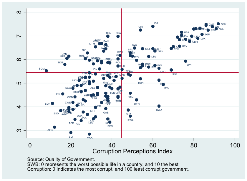
Figure 2. National average for subjective well-being and corruption perception in 2014

Table1

Summary Statistics: Mean of Main Variables

Variable	cpi_[25]	cpi_[50]	cpi_[75]	cpi_[100]	Total
National-Level Average Scores for Subjective Well-Being	4.51	5.08	5.31	6.57	5.45
Corruption Perception Index	21.89	30.84	43.56	73.68	44.64
Bayesian Corruption Index	63.24	58.38	50.92	30.29	49.50
Control of Corruption	-1.13	-0.75	-0.14	1.48	-0.04
Freedom from Corruption	18.09	25.72	37.87	74.25	40.91
Unemployment, Total (% of Total Labor Force)	6.99	6.66	9.98	8.15?	8.26
Natural logarithm (ln) of Capital Stock at Current purchasing power parity (PPP)	12.18	12.52	13.28	14.20	13.16
Average Exposure to PM2.5	90.29	91.75	86.69	91.02	89.56
GDP per Capita Growth (Annual %)	2.64	2.82	2.15	1.62	2.26
Population, Ages 15–64 (% of Total)	59.35	61.65	65.74	66.82	64.05
Religious Fractionalization	0.43	0.42	0.44	0.43	0.43
Ethnic Fractionalization	0.52	0.56	0.45	0.27	0.45
LanguageFractionalization	0.52	0.46	0.39	0.29	0.40

cpi_[25], cpi_[50], cpi_[75], and cpi_[100]represent the 25th, 50th, 75th, and 100th percentiles of the CPI, respectively. Data source: The Quality of Government Standard dataset, which draws on and compiles several freely available data sources, including the World Bank, TI, aggregated individual-level data, etc. PM2.5 is population-weighted exposure to fine particulate matter in micrograms per cubic meter that is 2.5 microns and smaller (3-year average) in a converted scale of 0 to 100, with 0 being the farthest from the target and 100 being closest to the target defined by established scientific consensus.

Table 2

The Effect of Corruption on Happiness, OLS and 2SLS

	Dependent Variable: National Average Scores for Subjective Well-Being
	OLS		2SLS
	(1)	(2)	(3)	(4)
CPI	0.039^***	0.026^***	0.042^***	0.023^**
	(0.0033)	(0.0034)	(0.0078)	(0.0099)
Unemployment Rate		-0.024^**		-0.025^***
		(0.0093)		(0.0093)
Ln of Capital Stock		0.17^***		0.17^***
		(0.033)		(0.040)
PM2.5		0.0084^**		0.0092^**
		(0.0036)		(0.0041)
GDP Growth Rate		-0.037		-0.040
		(0.024)		(0.025)
Working-Age Population		0.057^***		0.059^***
		(0.012)		(0.013)
Religious Fractionalization		0.057^***		-0.65^**
		(0.012)		(0.27)
Ethnic Fractionalization		-0.69^***		0.47
		(0.26)		(0.48)
Language Fractionalization		0.57		-0.51
		(0.38)		(0.38)
Underidentification			Reject^***(p-value: 0.000)	Reject^***(p-value:0.002)
Weak identification			Reject (CDW-F: 17.01;<10% size)	Reject (CDW-F:16.65; <10% size)
Observations	126	126	126	126
Adjusted R²	0.421	0.660	0.418	0.657

Robust standard errors are in parentheses. Data source: The Quality of Government Standard dataset. CPI comes originally from TI. It is a composite index based on a 0–100-point scale in which a score of 100 indicates very little corruption and a score of 0 indicates very high corruption in the public sector. The IV for CPI is preindustrial democracy in 2SLS regression. PM2.5 is population-weighted exposure to fine particulate matter in micrograms per cubic meter that is 2.5 microns and smaller (three-year average) in a converted scale of 0 to 100, with 0 being the farthest from the target and 100 being closest to the target defined by established scientific consensus.